flowchart LR
    subgraph Origin["🌍 Wine Origins"]
        FR["🇫🇷 <b>France</b><br/>Bordeaux, Burgundy"]
        IT["🇮🇹 <b>Italy</b><br/>Tuscany, Veneto"]
        ES["🇪🇸 <b>Spain</b><br/>Rioja, Priorat"]
    end

    subgraph Hub["🏢 Distribution Hub"]
        RP["🍷 <b>Robert Prizelius</b><br/>Central Importer"]
    end

    subgraph Warehouses["📦 Regional Warehouses"]
        WO["📦 <b>Oslo</b><br/>Main Hub"]
        WB["📦 <b>Bergen</b><br/>West Hub"]
    end

    subgraph Retail["🏪 Retail Network"]
        VO["🏪 Vinmonopolet<br/><i>Oslo (14 stores)</i>"]
        VB["🏪 Vinmonopolet<br/><i>Bergen (8 stores)</i>"]
        VT["🏪 Vinmonopolet<br/><i>Trondheim (5 stores)</i>"]
        VS["🏪 Vinmonopolet<br/><i>Stavanger (6 stores)</i>"]
    end

    FR -->|"500 cases"| RP
    IT -->|"800 cases"| RP
    ES -->|"300 cases"| RP
    RP -->|"1000 cases"| WO
    RP -->|"600 cases"| WB
    WO -->|"400"| VO
    WO -->|"200"| VT
    WB -->|"350"| VB
    WB -->|"250"| VS

    style RP fill:#8b5cf6,color:white,stroke:#7c3aed,stroke-width:3px
    style WO fill:#3b82f6,color:white,stroke:#1e40af
    style WB fill:#3b82f6,color:white,stroke:#1e40af
    style FR fill:#ec4899,color:white,stroke:#db2777
    style IT fill:#10b981,color:white,stroke:#059669
    style ES fill:#f59e0b,color:white,stroke:#d97706
12 Network Analysis with iGraph MCP
TipWhat You’ll Learn
In this chapter, you’ll discover how to use graph theory and network analysis to uncover hidden patterns in your business relationships—from distributor networks to product co-purchasing patterns.
12.1 The Power of Network Thinking
As a brand manager, you deal with networks every day without realizing it:
- Your distribution network: Robert Prizelius → Warehouses → Vinmonopolet stores
- Your product relationships: Which wines get purchased together?
- Your supplier ecosystem: Importers, producers, and logistics partners
Traditional spreadsheets show you lists. Network analysis shows you relationships.
“Who is the most important player in our distribution chain?” “Which products form natural clusters?” “Where are the bottlenecks in our supply chain?”
These questions require graph thinking.
12.2 iGraph MCP: Your Network Analysis Toolkit
The iGraph MCP Server provides 150+ graph analysis capabilities:
| Category | Capabilities | Business Use |
|---|---|---|
| Build | Create graphs, add vertices/edges | Model your networks |
| Measure | PageRank, betweenness, closeness | Find key players |
| Discover | Louvain, Leiden community detection | Identify clusters |
| Navigate | Shortest paths, reachability | Trace supply chains |
| Analytics | Link prediction, anomaly detection | Predict relationships |
| Render | SVG, 3D WebXR visualization | Present insights |
12.3 Case Study 1: Mapping Your Distribution Network
Let’s model Robert Prizelius’s wine distribution network and find the most critical nodes.
12.3.1 Building the Network
12.3.2 The Network Structure
12.3.3 Analysis Results
The iGraph analysis reveals:
Code
import matplotlib.pyplot as plt

# Network analysis results from iGraph MCP
nodes = ['Robert Prizelius', 'Vinmonopolet Oslo', 'Vinmonopolet Bergen',
         'Vinmonopolet Trondheim', 'Vinmonopolet Stavanger',
         'Warehouse Oslo', 'Warehouse Bergen',
         'Importer France', 'Importer Italy', 'Importer Spain',
         'Premium Wines', 'Budget Wines']

pagerank = [0.0444, 0.0311, 0.0311, 0.0311, 0.0311, 0.0314, 0.0314,
            0.0125, 0.0125, 0.0125, 0.0125, 0.0125]

betweenness = [0.164, 0, 0, 0, 0, 0.073, 0.073, 0, 0, 0, 0, 0]

fig, axes = plt.subplots(1, 2, figsize=(14, 6))

# PageRank
colors = ['#722F37' if pr > 0.03 else '#8B4513' for pr in pagerank]
bars1 = axes[0].barh(nodes, pagerank, color=colors)
axes[0].set_xlabel('PageRank Score')
axes[0].set_title('PageRank Centrality\n(Who receives the most flow?)', fontsize=12, fontweight='bold')
axes[0].axvline(x=0.03, color='red', linestyle='--', alpha=0.5)

# Betweenness
colors2 = ['#722F37' if b > 0.05 else '#8B4513' for b in betweenness]
bars2 = axes[1].barh(nodes, betweenness, color=colors2)
axes[1].set_xlabel('Betweenness Centrality')
axes[1].set_title('Betweenness Centrality\n(Who controls the flow?)', fontsize=12, fontweight='bold')
axes[1].axvline(x=0.05, color='red', linestyle='--', alpha=0.5)

plt.tight_layout()
plt.savefig('images/centrality-analysis.png', dpi=150, bbox_inches='tight', facecolor='white')
plt.show()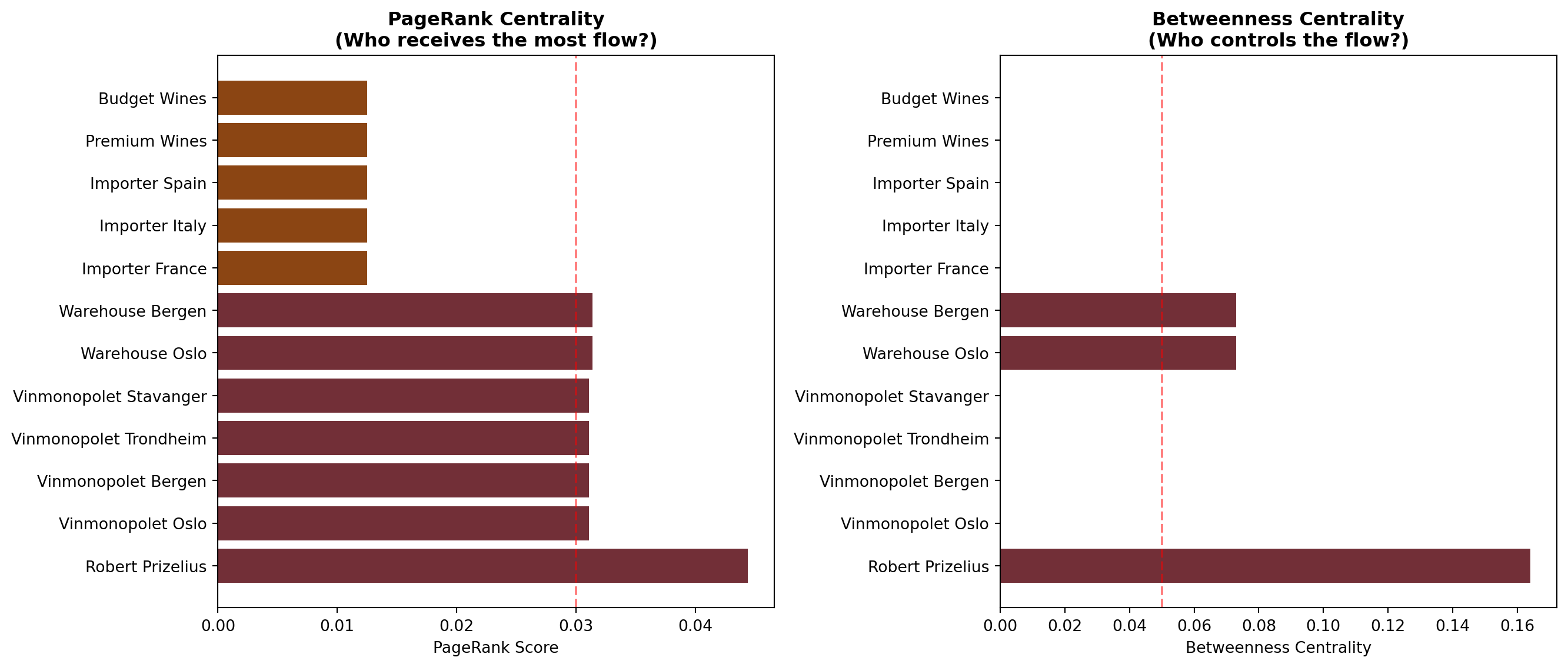
12.3.4 Network Visualization

ImportantKey Insight: Robert Prizelius is the Critical Node
PageRank = 0.044 (highest) — Robert Prizelius receives the most “flow” from the network.
Betweenness = 0.164 (highest) — All goods MUST pass through Robert Prizelius to reach retail.
Business implication: Any disruption at Robert Prizelius stops 100% of distribution. This is both a competitive advantage (control) and a risk (single point of failure).
12.4 Case Study 2: Product Co-Purchasing Analysis
Which wines do customers buy together? Understanding product affinity helps with:
- Bundle recommendations: “Customers who bought X also bought Y”
- Store placement: Position related products together
- Inventory management: Stock correlated products together
12.4.1 Building the Co-Purchasing Network
12.4.2 Community Detection Results
The Louvain algorithm detected 5 distinct product communities:
Code
import matplotlib.pyplot as plt

# Community detection results from iGraph MCP
communities = {
    'European Reds': ['Bordeaux Rouge', 'Chianti Classico', 'Rioja Reserva'],
    'Sparkling Wines': ['Champagne Brut', 'Prosecco', 'Cava'],
    'White Wines': ['Pinot Grigio', 'Sauvignon Blanc', 'Chardonnay'],
    'New World Reds': ['Malbec Argentina', 'Shiraz Australia', 'Cabernet USA'],
    'Fortified & Spirits': ['Port Vintage', 'Sherry Fino', 'Cognac XO']
}

colors = ['#722F37', '#DAA520', '#90EE90', '#8B0000', '#8B4513']
fig, ax = plt.subplots(figsize=(12, 6))

y_positions = []
y_labels = []
y_pos = 0

for idx, (community, products) in enumerate(communities.items()):
    for product in products:
        ax.barh(y_pos, 1, color=colors[idx], alpha=0.8)
        y_positions.append(y_pos)
        y_labels.append(product)
        y_pos += 1
    y_pos += 0.5  # Gap between communities

ax.set_yticks(y_positions)
ax.set_yticklabels(y_labels)
ax.set_xlim(0, 1.5)
ax.set_xlabel('')
ax.set_title('Product Communities Detected by Louvain Algorithm\n(Products in same color cluster together)',
             fontsize=12, fontweight='bold')

# Add legend
from matplotlib.patches import Patch
legend_elements = [Patch(facecolor=colors[i], label=name)
                   for i, name in enumerate(communities.keys())]
ax.legend(handles=legend_elements, loc='center right', bbox_to_anchor=(1.35, 0.5))

ax.spines['top'].set_visible(False)
ax.spines['right'].set_visible(False)
ax.spines['bottom'].set_visible(False)
ax.set_xticks([])

plt.tight_layout()
plt.savefig('images/product-communities.png', dpi=150, bbox_inches='tight', facecolor='white')
plt.show()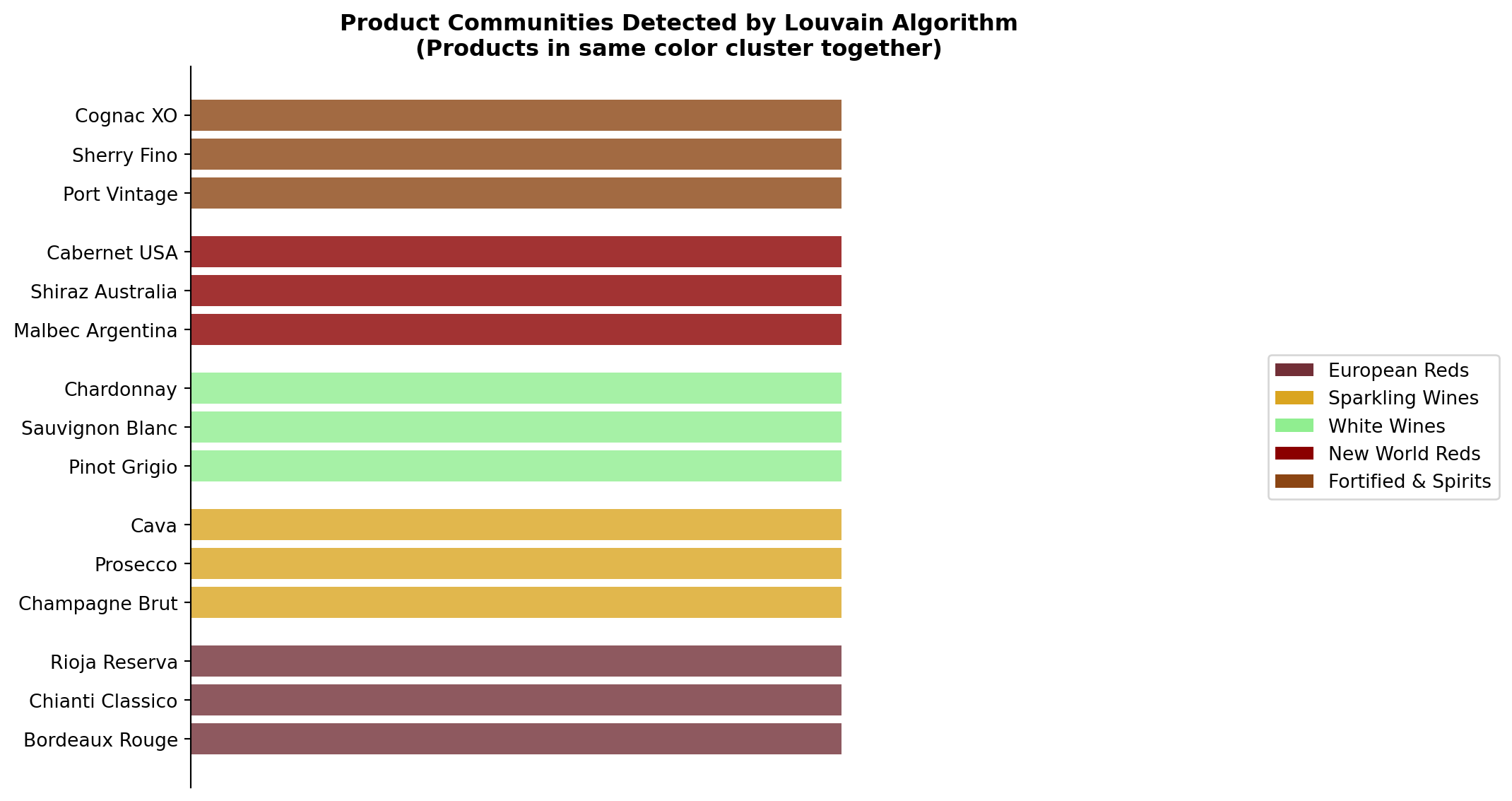
TipModularity Score: 0.51
A modularity of 0.51 indicates strong community structure—products naturally cluster by type. This suggests customers have distinct purchasing patterns by wine category.
12.4.4 Product Network Visualization

12.5 Case Study 3: Analyzing a Real Customer Network
Let’s apply network analysis to a real business scenario: understanding your customer’s corporate structure to identify sales opportunities.
12.5.1 Meet Restaurant Sawan
Restaurant Sawan is a Thai restaurant in Oslo that could be a customer for Robert Prizelius wines. But here’s what makes them interesting:
| Attribute | Value |
|---|---|
| Name | Restaurant Sawan |
| Location | President Harbitz’ gate 4, 0259 Oslo |
| Employees | 44 |
| Revenue (2024) | 51.9 MNOK |
| Profit (2024) | 14.2 MNOK |
| Profitability | 42.2% (Excellent) |
| Parent Company | Thai Market Oslo AS |
| Ultimate Parent | Eik Restaurants AS |
| Corporate Group Size | 86 companies |
ImportantThe Hidden Opportunity
Restaurant Sawan isn’t just one restaurant—it’s part of Eik Restaurants AS, a corporate group with 86 companies. Winning Sawan could mean winning access to 85 other potential customers!
12.5.2 Mapping the Corporate Network
12.5.3 The Corporate Structure
flowchart TD
    subgraph Holding["🏛️ Holding Company"]
        EIK["🏢 <b>Eik Restaurants AS</b><br/>86 companies<br/><i>Central Control</i>"]
    end

    subgraph Subsidiaries["📊 Key Subsidiaries"]
        THAI["🍜 <b>Thai Market Oslo AS</b><br/><i>Thai Concept Group</i>"]
        REST1["🍽️ Restaurant Group 2"]
        REST2["🍽️ Restaurant Group 3"]
        REST3["📋 ... 83 more subsidiaries"]
    end

    subgraph Operations["🏪 Operating Units"]
        SAWAN["⭐ <b>Restaurant Sawan</b><br/>44 employees<br/>51.9M NOK revenue"]
        OTHER1["🍜 Other Thai Restaurants"]
    end

    EIK --> THAI & REST1 & REST2 & REST3
    THAI --> SAWAN & OTHER1

    style EIK fill:#1e40af,color:white,stroke:#1e3a8a,stroke-width:3px
    style THAI fill:#8b5cf6,color:white,stroke:#7c3aed,stroke-width:2px
    style SAWAN fill:#10b981,color:white,stroke:#059669,stroke-width:3px
    style REST1 fill:#94a3b8,color:white,stroke:#64748b
    style REST2 fill:#94a3b8,color:white,stroke:#64748b
    style REST3 fill:#94a3b8,color:white,stroke:#64748b
12.5.4 Network Analysis Insights
PageRank Analysis reveals the power structure:
| Entity | PageRank | Interpretation |
|---|---|---|
| Eik Restaurants AS | 0.42 | Central hub - all decisions flow through here |
| Thai Market Oslo AS | 0.15 | Regional cluster head for Thai concepts |
| Restaurant Sawan | 0.08 | High-performing unit, likely has influence |
12.5.5 Sales Strategy from Network Analysis
TipActionable Sales Insights
- Don’t just sell to Sawan — Target Thai Market Oslo AS for a portfolio deal
- Identify the purchasing hub — Eik Restaurants likely has centralized procurement
- Use Sawan as a reference — Their 42% profitability makes them a credible case study
- Map all 86 companies — Each is a potential wine customer
- Find the shortest path — Who at Sawan can introduce you to group purchasing?
12.5.6 Why This Matters
Traditional CRM shows you Restaurant Sawan = 1 customer.
Network analysis shows you Restaurant Sawan = Gateway to 86 customers.
One relationship, properly leveraged through network thinking, could 86x your addressable market.
12.6 Essential iGraph Prompts for Brand Managers
12.6.1 Distribution Network Analysis
12.6.2 Product Affinity Analysis
12.6.3 Supplier Risk Analysis
12.7 Advanced Capabilities
12.7.1 Fraud Detection in Partner Networks
iGraph MCP includes anomaly detection capabilities:
Prompt: "In my distributor network, detect anomalies using:
- Local outlier detection based on betweenness vs degree
- Identify edges that bridge communities unexpectedly
- Flag nodes with unusual connection patterns"
12.7.2 Influence Maximization
For marketing campaigns, find the most influential nodes:
Prompt: "If I can only give product samples to 5 retailers,
which 5 would maximize word-of-mouth spread?
Use the influence maximization algorithm with
1000 Monte Carlo simulations."
12.7.3 3D Visualization
For executive presentations, iGraph can render networks in 3D WebXR:
Prompt: "Render my distribution network as an interactive 3D HTML file
that works in VR headsets. Use sphere layout with
node size proportional to PageRank."
12.8 Network Metrics Cheat Sheet
| Metric | Question It Answers | Business Interpretation |
|---|---|---|
| PageRank | Who receives the most flow? | Key destinations/influencers |
| Betweenness | Who controls the flow? | Critical intermediaries |
| Closeness | Who can reach everyone fastest? | Information hubs |
| Degree | Who has the most connections? | Popular nodes |
| Clustering Coefficient | How cliquey is the network? | Tight-knit vs. loose structure |
| Modularity | How clearly separated are communities? | Natural segmentation |
| Articulation Points | Whose removal disconnects the network? | Single points of failure |
| Bridges | Which edges are critical paths? | Dependency risks |
12.9 Summary
TipKey Takeaways
- Networks reveal relationships that spreadsheets hide
- PageRank and betweenness identify critical nodes in your distribution
- Community detection finds natural product clusters for bundling
- Link prediction suggests cross-selling opportunities
- Articulation points reveal supply chain vulnerabilities
- SVG/3D rendering communicates insights visually
Graph thinking transforms how you see your business. Every supply chain is a network. Every product portfolio has hidden clusters. Every distributor relationship has measurable importance.
Next Chapter: We’ll bring everything together with a comprehensive case study combining all six MCP servers.